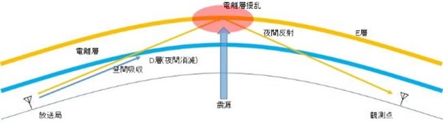
Fig.1 Radio wave propagation diagram of MF band AM broadcast waves
What ionospheric disturbance observation is
1. AM broadcast wave propagation
Fig.1 Radio wave propagation diagram of MF band AM broadcast waves
2. AM broadcast wave path and predicted epicenter area
As shown in Fig. 2, this method has the advantage of being able to cover
the entire Japan's epicenter area with a small number of observation points,
and making it easy to identify the predicted epicenter area.
For M=6 or less, the predicted epicenter area is assumed to
be a radius of 50 km from the center between the transmitting point and
the receiving point.
In order to observe the epicenter area throughout Japan without
any gaps, it is necessary to conduct observations in Sakhalin, Etorofu
Island, Taiwan, and the Philippines.
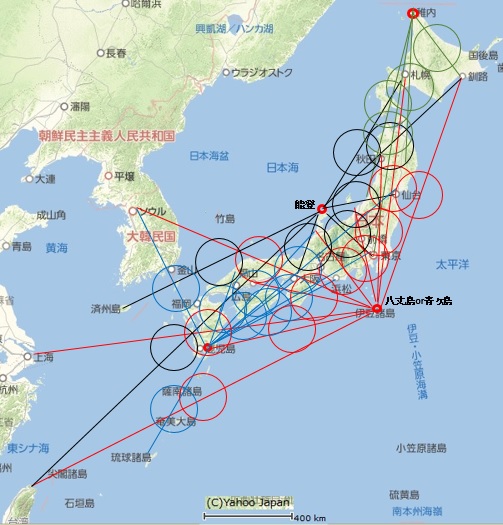
Fig.2 Nationwide observation using 4 domestic observation points
3. Example of ionospheric disturbance observation using AM broadcast waves
Fig. 3 shows an example of observation data for one day from Sapporo to
Sagamihara.
Fig. 4 shows an example of the standard deviation of variations
in morning and evening reception end and start times from Sapporo to Sagamihara
over the last four months.
Only four times did it exceed σ=2.
Figure 5 shows the predicted epicenter area on the path from
Sapporo to Sagamihara.
The predicted epicenter area is Akita Prefecture, western Iwate
Prefecture, and northern Miyagi Prefecture.
List-1 shows a list of earthquakes that occurred in the predicted
epicenter area within approximately one week from the day when σ exceeded
2.
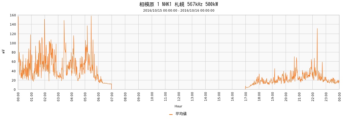
Fig.3 Data Graph for one day from Sapporo to Sagamihara
4. How to read the ionospheric disturbance observation statistical graph
-Green line graph: Morning Terminator Time (JST, left scale, hereinafter referred to as TT)
-Yellow line graph: Evening Terminator Time (JST, left scale)
-Green bar graph: Standard deviation of morning TT (σ Sigma, right scale)
-Orenge bar graph: Standard deviation of evening TT (σ Sigma, right scale)
-EQ: Occured Time of Noto Peninsula Earthquake (2024/1/1 16 : 10)
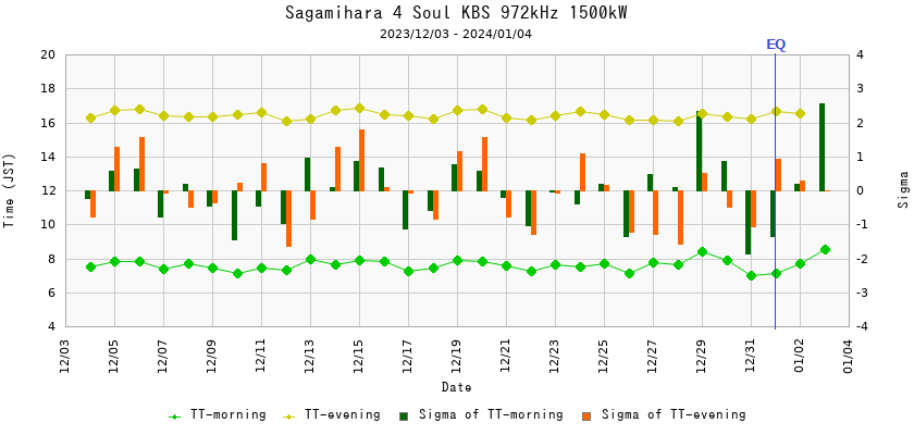
Fig.4 Standard deviation of morning and evening reception end/start time
fluctuations from Seoul to Sagamihara in the latest month
5. About standard deviation
(1) An easy-to-understand explanation of standard deviation is here
(2) The probability distribution (normal distribution) of data is expressed as shown below.
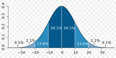
(Image source:wikipedia)
・The probability that the deviation from the average value is within ±1σ
is 68.27%, 95.45% when it is ±2σ or less, and 99.73%
when it is±3σ.
・A deviation of ±2σ is an anomaly that occurs only 4.55% of the time,
and a deviation of ±3σ is an anomaly that occurs only 0.27%.
・For the time being, the difference in the morning and evening reception
end/start times of medium-wave band AM broadcast waves
will be about ±2σ, and in 1 to 2 days it will be M=4 class, about
±3σ, If it continues for 1 to 2 days, it will be considered
as M=5 grade, and if it continues for 3 days or more, it will be
judged as M=6 grade or higher.
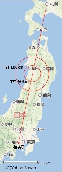
Fig.5 Predicted epicenter area on the path from Sapporo to Sagamihara
| σ>2 observed days | Earthquakes that occur in the predicted epicenter area within approximately one week | ||
| 6/30, 7/4 | 2016/7/16 22:12 | Northern inland area of Akita Prefecture | M4.6 |
| 8/18 | 2016/8/27 19:00 | Northern Miyagi Prefecture | M3.5 |
| 10/1, 2, 3 | 2016/10/10 8:15 | Northern inland area of Akita Prefecture | M3.2 |
| 10/12 | 2016/10/16 15:14 | Southern Miyagi Prefecture | M4.1 |
List-1 List of earthquakes that occurred in the predicted epicenter area
within one week from the day when σ exceeded 2
![]()
Please use all data and descriptions on this website at your own
risk.
Persons
affiliated with this center are not responsible for the results of using
this product.
Copyright (c)
Certified NPO Earthquake Precursor Observation Center (JEPCOC). All
rights reserved.